The world of artificial intelligence and machine learning has become increasingly accessible to newcomers, yet the concept of neural networks can still seem intimidatingly complex to those taking their first steps into this fascinating domain. Neural networks represent one of the most powerful and versatile tools in modern artificial intelligence, serving as the foundation for breakthrough technologies ranging from image recognition systems to natural language processing applications and autonomous vehicle navigation systems.
Understanding neural networks opens doors to comprehending how machines can learn patterns, make predictions, and solve complex problems that were once thought to be exclusively within the realm of human intelligence. This comprehensive guide will demystify the process of building your first neural network, breaking down complex concepts into digestible explanations and providing practical, hands-on experience that transforms theoretical knowledge into applicable skills.
Explore the latest AI developments and neural network innovations to stay current with rapidly evolving machine learning technologies that continue to reshape industries and create new possibilities for intelligent automation. The journey from understanding basic neural network concepts to implementing functional models represents a crucial step in developing expertise in artificial intelligence and machine learning applications.
Understanding Neural Networks: The Foundation
Neural networks draw inspiration from the biological neural networks found in animal brains, particularly the human brain, where interconnected neurons process and transmit information through electrical and chemical signals. Artificial neural networks attempt to replicate this information processing mechanism using mathematical models and computational algorithms that can learn from data and make intelligent decisions based on learned patterns.
At its core, a neural network consists of layers of interconnected nodes called neurons or perceptrons, each designed to receive input signals, process them through mathematical functions, and produce output signals that serve as inputs for subsequent layers. The fundamental principle underlying neural network functionality involves the concept of weighted connections between neurons, where these weights are adjusted during the learning process to optimize the network’s ability to produce desired outputs for given inputs.
The power of neural networks lies in their ability to approximate complex mathematical functions and identify intricate patterns within large datasets without requiring explicit programming for each specific scenario. This capability emerges from the network’s architecture and the iterative training process that gradually refines the connection weights through exposure to training examples and feedback mechanisms that guide the learning process toward improved performance.
Essential Components and Architecture
Every neural network comprises several fundamental components that work together to process information and generate meaningful outputs. The input layer serves as the entry point for data, where each neuron represents a specific feature or dimension of the input data, such as pixel values in an image or individual words in a text document. These input neurons simply pass the received data to the next layer without performing any mathematical transformations.
Hidden layers represent the computational heart of the neural network, where the actual learning and pattern recognition occur through complex mathematical operations. Each neuron in a hidden layer receives weighted inputs from all neurons in the previous layer, applies an activation function to the sum of these weighted inputs, and produces an output that becomes an input for neurons in the subsequent layer. The number of hidden layers and the number of neurons within each layer significantly influence the network’s capacity to learn complex patterns and relationships.
The output layer produces the final results of the neural network’s computations, with the number of output neurons corresponding to the specific task requirements. For binary classification problems, a single output neuron might suffice, while multi-class classification tasks require multiple output neurons, each representing the probability of belonging to a specific class. Regression problems typically utilize a single output neuron that produces continuous numerical values.
Activation functions play a crucial role in introducing non-linearity into the neural network, enabling it to learn complex patterns that cannot be captured by simple linear relationships. Common activation functions include the sigmoid function, which maps inputs to values between zero and one, the hyperbolic tangent function that produces outputs between negative one and positive one, and the rectified linear unit function that outputs the input value for positive inputs and zero for negative inputs.
The Mathematics Behind Neural Networks
The mathematical foundation of neural networks centers around linear algebra operations, particularly matrix multiplication and vector operations that efficiently process multiple inputs simultaneously. Each connection between neurons has an associated weight that determines the strength and direction of the influence that one neuron exerts on another. These weights are organized into matrices that facilitate efficient computation of the entire network’s operations through matrix multiplication.
The forward propagation process involves computing the output of each layer sequentially, starting from the input layer and proceeding through hidden layers to reach the output layer. For each neuron, the computation involves calculating the weighted sum of inputs, adding a bias term that allows the activation function to shift, and applying the activation function to produce the neuron’s output. This process can be expressed mathematically as the composition of linear transformations followed by non-linear activation functions.
Enhance your understanding with advanced AI tools like Claude to explore complex mathematical concepts and receive detailed explanations of neural network operations, optimization algorithms, and advanced architectures. The mathematical elegance of neural networks becomes apparent when viewed through the lens of optimization theory, where the goal is to minimize a loss function that quantifies the difference between predicted and actual outputs.
The backpropagation algorithm represents the cornerstone of neural network training, utilizing the chain rule of calculus to compute gradients of the loss function with respect to each weight in the network. These gradients indicate the direction and magnitude of weight adjustments needed to reduce the loss function, enabling the optimization algorithm to iteratively improve the network’s performance through gradient descent or more sophisticated optimization techniques.
Setting Up Your Development Environment
Before diving into neural network implementation, establishing a proper development environment ensures smooth progress and access to necessary tools and libraries. Python has emerged as the preferred programming language for machine learning and neural network development due to its simplicity, extensive library ecosystem, and strong community support. Installing Python through the Anaconda distribution provides a comprehensive package management system and pre-configured environment for scientific computing.
Essential libraries for neural network development include NumPy for numerical computations and array operations, Matplotlib for data visualization and plotting results, and either TensorFlow or PyTorch as the primary deep learning framework. TensorFlow, developed by Google, offers high-level APIs through Keras that simplify neural network construction and training, while PyTorch, developed by Facebook, provides dynamic computational graphs and intuitive debugging capabilities.
Setting up a virtual environment isolates your neural network projects from other Python installations and prevents dependency conflicts that might arise from different project requirements. Virtual environments ensure reproducible results and facilitate sharing your code with others who can recreate the exact same computational environment needed to run your neural network implementations.
Jupyter Notebooks provide an excellent interactive development environment for experimenting with neural networks, allowing you to combine code execution, visualization, and documentation in a single interface. This environment facilitates iterative development and experimentation, enabling you to modify network architectures, adjust hyperparameters, and visualize results without the overhead of traditional script-based development workflows.
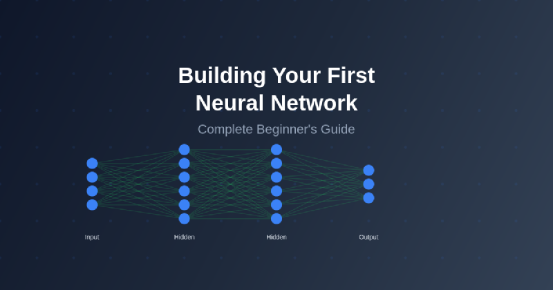
Building Your First Neural Network
The journey of building your first neural network begins with a simple yet illustrative problem that demonstrates fundamental concepts without overwhelming complexity. A classic starting point involves creating a binary classification network that can distinguish between two categories, such as determining whether an email is spam or legitimate, or classifying images as containing cats or dogs.
Starting with a basic feedforward neural network architecture provides solid foundations for understanding more complex architectures later. This initial network typically consists of an input layer dimensioned according to your data features, one or two hidden layers with a moderate number of neurons, and an output layer appropriate for your specific task. The simplicity of this architecture allows focus on understanding the core mechanics without getting lost in architectural complexity.
The implementation process begins with data preparation, where raw data is transformed into a format suitable for neural network processing. This preprocessing typically involves normalizing numerical features to similar scales, encoding categorical variables into numerical representations, and splitting the dataset into training, validation, and testing subsets to ensure proper evaluation of the network’s performance and generalization capabilities.
Defining the network architecture involves specifying the number of layers, neurons per layer, activation functions, and connection patterns between layers. Most deep learning frameworks provide high-level APIs that abstract away low-level implementation details, allowing you to focus on architectural decisions rather than mathematical implementation complexities. The initial architecture serves as a starting point that can be refined based on performance observations and experimentation.
Training Process and Optimization
The training process transforms a randomly initialized neural network into a functional model capable of making accurate predictions through iterative exposure to training examples and systematic weight adjustments. This process begins with forward propagation, where training examples are fed through the network to produce predictions, followed by loss computation that quantifies the difference between predicted and actual outputs.
The choice of loss function significantly impacts the training process and final performance characteristics. Binary classification problems typically utilize binary cross-entropy loss, while multi-class classification employs categorical cross-entropy, and regression tasks often use mean squared error. The loss function serves as the objective that the optimization algorithm attempts to minimize through systematic weight adjustments.
Backpropagation computes gradients of the loss function with respect to each network parameter, providing the information needed to adjust weights in directions that reduce the loss. These gradients flow backward through the network, starting from the output layer and propagating through hidden layers to the input layer, hence the name backpropagation. The chain rule of calculus enables efficient computation of these gradients for networks of arbitrary depth.
Optimization algorithms determine how the computed gradients are used to update network weights. Stochastic gradient descent represents the simplest approach, adjusting weights proportionally to the computed gradients with a learning rate parameter controlling the step size. More sophisticated optimizers like Adam, RMSprop, and AdaGrad incorporate momentum and adaptive learning rates to improve convergence speed and stability during training.
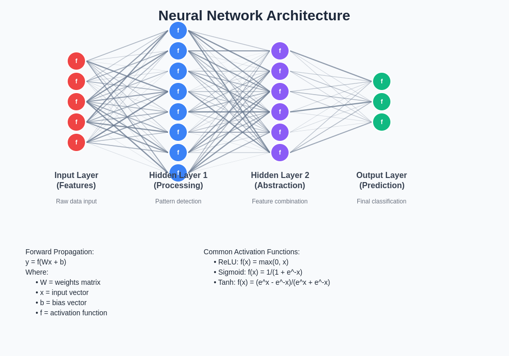
The architecture visualization illustrates the fundamental structure of a neural network, showing how information flows from input features through hidden layers to produce final outputs. Understanding this information flow is crucial for grasping how neural networks process data and learn complex patterns through interconnected computational units.
Hyperparameter Tuning and Optimization
Hyperparameters represent the configuration settings that control the neural network’s architecture and training process, distinct from the learnable parameters that are adjusted during training. These hyperparameters significantly influence the network’s ability to learn effectively and generalize to new, unseen data. Key architectural hyperparameters include the number of hidden layers, neurons per layer, and choice of activation functions.
Learning rate stands as one of the most critical hyperparameters, controlling the step size used during weight updates. A learning rate that is too high can cause the training process to overshoot optimal solutions and fail to converge, while a learning rate that is too low results in extremely slow convergence and may get stuck in local minima. Finding the optimal learning rate often requires experimentation and may benefit from adaptive scheduling that adjusts the rate during training.
Batch size determines how many training examples are processed simultaneously during each weight update. Larger batch sizes provide more stable gradient estimates but require more memory and may lead to convergence to sharper minima that generalize poorly. Smaller batch sizes introduce more noise into the training process but can help escape local minima and often lead to better generalization performance.
Regularization techniques help prevent overfitting, where the network memorizes training data rather than learning generalizable patterns. Common regularization approaches include dropout, which randomly deactivates neurons during training to prevent over-reliance on specific connections, and weight decay, which penalizes large weight values to encourage simpler, more generalizable models.
Discover powerful AI research capabilities with Perplexity to explore advanced hyperparameter optimization techniques, automated machine learning approaches, and cutting-edge research in neural network architecture design. The systematic exploration of hyperparameter spaces can significantly improve model performance and requires understanding of the trade-offs between different configuration choices.
Common Challenges and Solutions
Beginning neural network practitioners encounter several common challenges that can impede progress and lead to frustration. Overfitting represents one of the most frequent issues, where the network performs excellently on training data but fails to generalize to new examples. This problem typically manifests as a growing gap between training and validation performance during the training process.
Addressing overfitting requires implementing regularization strategies, reducing model complexity, or increasing the amount of training data. Early stopping monitors validation performance during training and halts the process when validation loss begins to increase, preventing the network from continuing to memorize training examples. Data augmentation artificially increases dataset size by creating modified versions of existing examples, providing more diverse training material.
Vanishing gradients pose challenges in deeper networks, where gradients become progressively smaller as they propagate backward through many layers, effectively preventing early layers from learning meaningful representations. This problem can be mitigated through careful initialization strategies, batch normalization that stabilizes the distribution of layer inputs, and architectural choices like residual connections that provide alternative gradient flow paths.
Conversely, exploding gradients can cause training instability when gradients become extremely large, leading to dramatic weight updates that destabilize the learning process. Gradient clipping provides a simple solution by limiting gradient magnitudes to reasonable ranges, while proper weight initialization and learning rate selection can prevent the problem from occurring.
Practical Implementation Example
Implementing a concrete neural network example solidifies theoretical understanding through hands-on experience. Consider building a network to classify handwritten digits from the MNIST dataset, a classic benchmark problem that provides an excellent introduction to image classification with neural networks. This problem involves recognizing digits zero through nine from grayscale images containing handwritten numerals.
The implementation begins with data loading and preprocessing, where the MNIST dataset is downloaded and prepared for neural network consumption. Images are normalized to ensure pixel values fall within a consistent range, typically between zero and one, and labels are converted to one-hot encoded vectors that represent each digit as a binary vector with a single active element.
Network architecture for this problem typically involves flattening the two-dimensional image into a one-dimensional vector that serves as input to a fully connected network. A simple yet effective architecture might include an input layer with 784 neurons corresponding to the flattened image pixels, one or two hidden layers with several hundred neurons each, and an output layer with ten neurons representing the probability of each digit class.
The training process involves compiling the model with appropriate loss function, optimizer, and evaluation metrics, followed by iterative training on batches of examples. Monitoring training progress through loss and accuracy metrics provides insights into the network’s learning behavior and helps identify when training should be stopped to prevent overfitting.
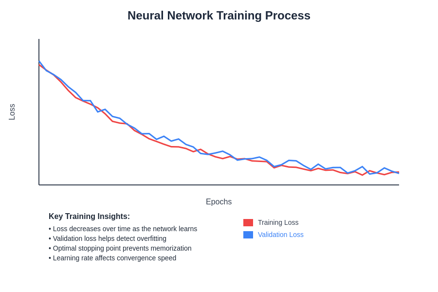
The training visualization demonstrates how loss decreases and accuracy improves over training epochs, illustrating the learning process and helping identify optimal stopping points to prevent overfitting while maximizing performance on validation data.
Evaluating Model Performance
Proper evaluation of neural network performance extends beyond simple accuracy measurements to provide comprehensive understanding of model capabilities and limitations. Training accuracy indicates how well the network has learned the training data, but validation accuracy provides a more reliable estimate of performance on unseen examples and serves as a better predictor of real-world performance.
Confusion matrices offer detailed insights into classification performance by showing the distribution of predicted versus actual classes. This visualization reveals which classes the network confuses most frequently and helps identify systematic biases or weaknesses in the learned representations. For multi-class problems, confusion matrices can reveal whether certain classes are consistently misclassified as specific other classes.
Precision and recall metrics provide additional perspectives on classification performance, particularly important for imbalanced datasets where simple accuracy can be misleading. Precision measures the fraction of positive predictions that are actually correct, while recall measures the fraction of actual positive examples that are correctly identified. The F1-score combines precision and recall into a single metric that balances both considerations.
Learning curves plot training and validation performance metrics over training epochs, providing visual insights into the learning process and helping identify overfitting, underfitting, or optimal stopping points. These curves can reveal whether the network would benefit from additional training data, different architectural choices, or alternative regularization strategies.
Advanced Concepts and Next Steps
Having mastered the fundamentals of neural network construction and training, several advanced concepts await exploration to deepen understanding and expand capabilities. Convolutional Neural Networks represent a specialized architecture particularly effective for image processing tasks, utilizing convolution operations that preserve spatial relationships and reduce the number of parameters needed for image analysis.
Recurrent Neural Networks excel at processing sequential data such as time series, natural language, or any data where temporal relationships matter. These networks maintain internal state that allows them to remember information from previous inputs, enabling them to model dependencies across time steps and capture patterns in sequential data.
Transfer learning leverages pre-trained networks that have already learned useful representations on large datasets, allowing you to adapt these learned features to new tasks with limited training data. This approach significantly reduces training time and often achieves better performance than training from scratch, particularly when working with small datasets.
Ensemble methods combine predictions from multiple neural networks to achieve better performance than any individual network. Techniques like bagging, boosting, and stacking can be applied to neural networks to reduce overfitting, improve generalization, and increase robustness to individual model weaknesses.
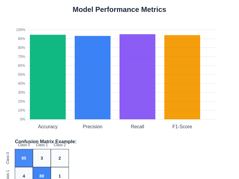
The performance comparison illustrates how different neural network configurations and techniques affect various evaluation metrics, helping guide architectural decisions and optimization strategies for achieving optimal results across different performance dimensions.
Best Practices and Professional Development
Developing professional-level neural network implementations requires adherence to software engineering best practices and machine learning workflow standards. Version control systems like Git help track changes to model architectures, hyperparameter configurations, and training scripts, enabling reproducible experiments and collaborative development with team members.
Experiment tracking tools facilitate systematic exploration of different model configurations by automatically logging hyperparameters, training metrics, and model artifacts. These tools help identify successful configurations, avoid repeating failed experiments, and maintain comprehensive records of model development progress.
Code organization and documentation become increasingly important as neural network projects grow in complexity. Modular code design separates data preprocessing, model definition, training loops, and evaluation procedures into distinct components that can be tested independently and reused across different projects.
Continuous learning remains essential in the rapidly evolving field of neural networks and deep learning. Following research publications, participating in online communities, and experimenting with new architectures and techniques help maintain current knowledge and develop expertise in emerging areas of artificial intelligence and machine learning.
The journey from building your first neural network to developing sophisticated deep learning applications requires patience, practice, and persistent experimentation. Each project provides opportunities to deepen understanding, encounter new challenges, and develop the intuition needed to design effective solutions for complex real-world problems.
Troubleshooting and Debugging
Debugging neural networks requires systematic approaches to identify and resolve issues that can arise during development and training. Common symptoms of problematic networks include failure to converge during training, poor performance on validation data, or unstable training behavior characterized by erratic loss fluctuations.
Network architecture issues often manifest as consistently poor performance regardless of training duration or hyperparameter adjustments. These problems might indicate insufficient network capacity for the problem complexity, inappropriate activation functions, or architectural mismatches between the problem structure and network design. Systematic experimentation with different architectures helps identify optimal configurations.
Data-related problems frequently cause training difficulties and poor generalization performance. Issues such as inconsistent data preprocessing, incorrect label encoding, or data leakage between training and validation sets can significantly impact network performance. Careful data inspection and validation help identify and resolve these fundamental issues.
Training instabilities often result from inappropriate hyperparameter choices, particularly learning rates that are too high or optimization algorithms that are poorly suited to the specific problem characteristics. Monitoring training metrics closely and adjusting hyperparameters based on observed behavior helps stabilize the training process and achieve better convergence.
Future Directions and Emerging Trends
The field of neural networks continues to evolve rapidly, with new architectures, training techniques, and applications emerging regularly. Transformer architectures have revolutionized natural language processing and are increasingly being applied to computer vision and other domains, demonstrating the power of attention mechanisms for capturing complex relationships in data.
Automated machine learning approaches aim to democratize neural network development by automatically searching for optimal architectures and hyperparameters, reducing the expertise required to develop effective models. These techniques promise to make neural network development accessible to practitioners without deep machine learning expertise.
Federated learning enables training neural networks across distributed datasets without centralizing data, addressing privacy concerns and enabling collaboration across organizations while maintaining data sovereignty. This approach opens new possibilities for training on sensitive datasets and scaling machine learning to global applications.
The integration of neural networks with other artificial intelligence techniques creates hybrid systems that combine the pattern recognition capabilities of deep learning with the reasoning abilities of symbolic AI, promising more robust and interpretable intelligent systems for complex real-world applications.
Building your first neural network represents the beginning of an exciting journey into the world of artificial intelligence and machine learning. The foundational knowledge gained through this comprehensive guide provides the stepping stones for exploring advanced architectures, tackling complex problems, and contributing to the ongoing revolution in intelligent systems that continue to transform industries and create new possibilities for human-machine collaboration.
Disclaimer
This article is for educational purposes only and does not constitute professional advice. The implementation examples and techniques described should be adapted to specific use cases and requirements. Neural network development involves experimentation and iteration, and results may vary based on data characteristics, problem complexity, and implementation details. Readers should conduct thorough testing and validation before deploying neural networks in production environments.